Methodology: Location based financial metrics (1/2)
To provide a forward-looking and financially relevant assessment of climate risk, we use a two-step methodology to quantify the nuances of climate's financial impacts on different asset types:
- Location-Based Physical Risk: First, we calculate a set of asset-agnostic metrics for a specific geographic location. These translate raw climate data (e.g., changes in temperature, precipitation) into standardized measures of baseline physical risk. This layer answers the question: "What is the baseline climate exposure at this location?"
- Asset-Specific Vulnerability Adjustment: Second, we adjust the baseline geographic risk using evidence-based Sensitivity Coefficients to reflect the unique vulnerabilities of a specific asset class. This layer answers the question: "How does this specific asset (e.g., a data center vs. a residential building) actually experience the baseline risk at this location?"
The relationship between these layers forms the core of our analysis:
Final_Impact_Asset = Baseline_Impact_Geo × f(Sensitivity_Coefficient)
The metric formulas below describe the location-based calculation. Asset-type multipliers are applied through the shared adjustment above to obtain the final asset impact. The next page explains that asset-specific vulnerability framework.
Section 1 — Valuation
1.1 10-Year NPV Loss (CVaR)
This figure represents the expected Net Present Value (NPV) loss under adverse but plausible climate scenarios (Climate Value at Risk, or CVaR).
Rather than a standalone variable, CVaR is a top-level aggregate metric calculated using a standard Discounted Cash Flow (DCF) model over a 10-year holding period. We project a baseline scenario (assuming no new climate impacts) and compare it against a climate-stressed scenario. The climate-stressed scenario incorporates our forecast for all the bottom-up features discussed below—such as increased insurance premiums, higher maintenance costs, required retrofits (CapEx), and reductions in income.
The total percentage difference between the baseline NPV and the climate-stressed NPV over this 10-year period is the 10-Year NPV Loss. For an easy-to-understand demonstration of this calculation (using a simplified 5-year example), see our DCF Use Case.
1.2 Average Annual Loss (AAL)
The Average Annual Loss (AAL) represents the all-in annualized cost of climate exposure. Because the 10-Year NPV Loss (CVaR) represents a cumulative impact over a decade, the AAL simply translates this total reduction into an averaged annualized value. This provides asset managers with a straightforward metric showing the expected percentage of asset value lost each year due to the aggregated climate-driven OpEx, CapEx, and revenue impacts.
1.3 Climate Risk Discount
Climate Risk Discount translates a location’s future resilience-adjusted physical risk into an adjustment to its exit capitalization rate. The calculation scales the combined impact across nine hazards against the global reference range for each horizon, using reference rates of 0.8% for 2035, 1.2% for 2050 and 2.0% for 2100. These are reference scaling rates, not enforced upper limits.
For example, a 0.25-percentage-point adjustment increases a 5% exit cap rate to 5.25%, reducing terminal value. The DCF discount rate remains unchanged.
.png)
Kernel Density Distribution of location climate discount rates for all locations in the world. Most locations/assets experience minimal correction, while locations in highly risky areas are shown to have high tail risks.
1.4 Adaptation Alpha
While the metrics above quantify the financial losses from climate risk, Adaptation Alpha quantifies the financial opportunity — the portion of projected NPV loss that is recoverable if targeted, building-level adaptation measures are implemented. It answers the question: "How much asset value can be defended by adapting this building to its climate exposure?"
Like the 10-Year NPV Loss (CVaR), Adaptation Alpha is a top-level aggregate metric built on the same Discounted Cash Flow (DCF) model over a 10-year holding period. Here we project three scenarios and compare them:
- Base NPV — the baseline scenario assuming no new climate impacts.
- Unadapted NPV — the climate-stressed scenario incorporating all bottom-up impacts (insurance, OpEx, CapEx, income, and the Climate Risk Discount). This is identical to the climate-stressed case used for the 10-Year NPV Loss.
- Adapted NPV — the same climate-stressed scenario, but with each climate impact reduced to reflect the resilience benefit of adaptation measures already in place (or being considered) at the asset.
Adaptation Alpha is the value recovered by adaptation, expressed as a percentage of Base NPV:
Adaptation_Alpha = (Adapted_NPV − Unadapted_NPV) / Base_NPV × 100
Equivalently, it is the reduction in projected NPV loss: an asset facing a 10-year unadapted loss of, say, 8% might face only a 3% loss once adapted — a recovered +5% of asset value.
How adaptation reduces climate impact
The adaptation benefit is derived from a resilience questionnaire covering building- and site-level strategies (e.g. wind-rated structure, elevated utilities, flood barriers, fire-resistant materials, passive cooling, drought-tolerant landscaping). Each strategy is weighted by its impact (Low = 1, Medium = 2, High = 3) against the 9 hazards that drive financial risk: Heat Stress, Drought, Hurricane Wind, Inland Flooding, Coastal Flooding, Wildfire, Hail, Landslide, and Earthquake.
For each hazard, a reduction factor is calculated as the share of available resilience points earned by the adaptation measures in place, scaled by a maximum cap:
Reduction_Factor_hazard = (Earned_Points / Max_Possible_Points) × Max_Reduction_Cap
The maximum reduction is capped at 70% — adaptation mitigates, but never fully eliminates, climate exposure. Strategies that are not applicable to a location are excluded from the denominator so that the factor reflects only relevant defenses.
For DCF parameters that use an average hazard reduction, the adjustment is Adapted_Impact = Unadapted_Impact × (1 − avg_reduction). Insurance is recalculated from the adapted inland-flood, coastal-flood and wildfire impacts: each peril's reduction factor is applied to both its 2025 and 2050 inputs, and the insurance-growth formula below is run again. This does not imply a proportional reduction in the growth rate; scaling both impacts can leave their ratio unchanged above the baseline floor.
Hazard → financial impact mapping:
| Hazard | DCF impacts reduced by adaptation |
|---|---|
| Heat Stress | Utility demand, operational efficiency, downtime, workforce productivity, Climate Risk Discount |
| Drought | Operational downtime, Climate Risk Discount |
| Hurricane Wind | Retrofit CapEx, downtime, maintenance, Climate Risk Discount |
| Inland Flooding | Retrofit CapEx, insurance premiums, Climate Risk Discount |
| Coastal Flooding | Retrofit CapEx, insurance premiums, Climate Risk Discount |
| Wildfire | Retrofit CapEx, insurance premiums, Climate Risk Discount |
| Hail | Retrofit CapEx, maintenance, Climate Risk Discount |
| Landslide | Retrofit CapEx, Climate Risk Discount |
| Earthquake | Retrofit CapEx, Climate Risk Discount |
By default, the metric reports the best-case opportunity (all relevant strategies adopted). When a specific asset's resilience profile is supplied, the reduction factors — and therefore the recoverable value — reflect only the measures actually in place, allowing users to compare the value at stake against the cost of closing the adaptation gap.
Section 2 — Insurance
2.1 Insurance Premiums
The insurance premium metric estimates annualized climate-driven premium growth between 2025 and 2050 from three perils: inland flooding, coastal flooding and wildfire. It uses each peril's resilience-adjusted impact at the location. Results are expressed as annual percentage rates.
Methodological grounding
Insurance ratemaking links premiums to expected claims, expenses and a profit provision. CAS Basic Ratemaking, Chapters 1 and 8, describes this relationship and the pure-premium and loss-ratio approaches. This provides the economic rationale for using changes in physical damage potential to indicate pressure on the risk-related component of insurance premiums. AlphaGeo uses resilience-adjusted impact growth as a proxy for that pressure.
Catastrophe risk requires attention to the frequency, severity and geographic distribution of events. ASOP No. 39, Sections 3.3–3.4, recognises the use of noninsurance data and models when claims experience does not adequately represent catastrophe exposure. This supports using modelled hazard information to assess changing risk. In flood insurance, FEMA's Risk Rating 2.0 provides a practical example of property-level risk informing premiums; GAO's 2023 assessment found that the approach improved their alignment with flood risk.
There is also empirical evidence of an association between climate exposure and premiums. The U.S. Treasury's 2025 homeowners-insurance analysis found higher average premiums in ZIP codes with higher expected losses from climate-related perils. That study excludes flood coverage; the FEMA/GAO evidence provides the separate flood-insurance context.
How this informs the calculation
The model compares 2025 and 2050 resilience-adjusted impacts to express the change in damage potential over a common long-term horizon. Annualizing that change gives a constant compound rate that can be used in cashflow modelling. The 25-year interval expresses the scenario's long-term change; it does not describe the timing of individual annual renewals.
Calculation
For each peril h:
g_h = (1 + max(R2050_h − R2025_h, 0)
             / max(R2025_h, epsilon_h))^(1/25) − 1

INS_RATE_h      = 100 × g_h
INS_RATE_FLOOD  = INS_RATE_INLAND + INS_RATE_COASTAL
INS_RATE_ANNUAL = INS_RATE_FLOOD + INS_RATE_FIRE
R2025_handR2050_hare the peril's resilience-adjusted impact values before conversion to the displayed risk score. These are impact proxies; they carry no insured-loss currency amount.epsilon_his a denominator floor of 1 impact point for each peril. It keeps the calculation finite where baseline impact is zero or very small.- The exponent annualizes the change over the 25 years from 2025 to 2050. Multiplication by 100 expresses each contribution as an annual percentage rate. For example, a returned value of 2 means 2% per year.
Above the baseline floor, an increase from 10 to 20 impact points produces approximately 2.81% annual growth for that peril. Other peril contributions are then added to obtain the total.
How to interpret the result
Stable or declining impact contributes zero growth. A location with high but stable exposure can therefore have a low insurance-growth estimate. Read this metric alongside the location's risk profile. A decrease in a peril's impact does not generate a negative premium-growth contribution in this model.
Scope and methodological limits
The metric estimates the climate-driven component of insurance premium growth over 2025–2050. Observed premium growth can differ because of rebuilding-cost inflation, insurer competition and capacity, reinsurance costs, regulation, and changes in coverage or deductibles. These influences on pricing are discussed in CAS Basic Ratemaking, Chapters 6, 7 and 13.
The 25-year horizon focuses on long-term changes in climate risk. Cyclical pricing pressures may moderate over time, but persistent changes in rebuilding costs, insurance capacity or regulation can sustain differences between observed premiums and the climate-driven projection.
To help users interpret these differences, we provide historical rebuilding-cost inflation and insurance premium trends at the sub-market level where available. These references show local cost and pricing conditions alongside the climate projection, with their available observation periods and geographic coverage.
Contributing features
| Peril | Input | Contribution |
|---|---|---|
| Inland flooding | Resilience-adjusted inland-flood impacts for 2025 and 2050 | Inland component of flood-related premium growth |
| Coastal flooding | Resilience-adjusted coastal-flood impacts for 2025 and 2050 | Coastal component of flood-related premium growth |
| Wildfire | Resilience-adjusted wildfire impacts for 2025 and 2050 | Fire-related premium growth |
2.2 Insurability Risk
In certain high-risk locations, the probability and severity of climate-related damages may become so extreme that the risk is technically or economically uninsurable. This metric provides a simple binary flag to identify such locations by testing if their future risk level will surpass what is considered an extreme outlier in today's market.
To acheive this, a location is flagged as uninsurable if its future risk score exceeds the 99th percentile of the current risk distribution.
Uninsurable = 1 if OVERALL_IMPACT_2050 > P99(OVERALL_IMPACT_2025)
| Feature | Description | Rationale | Unit |
| OVERALL_IMPACT_2025 | The blended physical risk impact score for 2025 from a global or continental distribution. | The 99th percentile of this score represents the current market's threshold for an extreme, potentially uninsurable, level of risk. | Index |
| OVERALL_IMPACT_2050 | The blended physical risk impact score for 2050 for a specific location. | This is the future risk level that is tested against the current market's insurability threshold. | Index |
Section 3 — OpEx Costs
3.1 Utility Demand
The utility demand component estimates the expected annual increase in heating and cooling costs experienced by an asset using the changes of cooling and heating degree days.
The cooling and heating requirement to keep occupants comfortable is expected over time due to climate change. By comparing the percentage increase (or decrease) between the cooling/heating demand of the baseline year (currently 2025) and future the future year (2050), we can then obtain the annual change of heat and cooling demand of a building.
Cooling demand calculation
The effective cooling demand of a location are calculated from Cooling Degree Days (CDD) which are a proxy to that measures the demand for energy to cool buildings to a comfortable temperature for its occupants. This is achieved using two different equations, with the maximum value taken as the final CDD value.
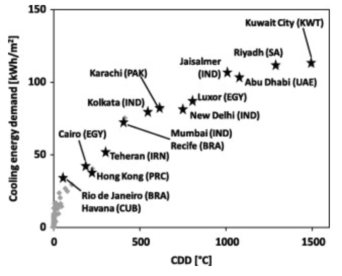
Relationship between cooling demand and CDD according to De Rosa, Mattia, et al.
Eqn1 (Applicable in locations with CDD > 200): cooling energy demand kWh/m2 = cdd * 0.0193-2.913
Eqn2 (Applicable for all locations): cooling energy demand kWh/m2 = cdd * 0.09 + 2.8
Heating demand calculation
Heating Degree Days (HDD) are a proxy to that measures the demand for energy to heat buildings to a comfortable temperature for its occupants. The effective heating demand is calculated using a single equation derived from published literature. This equation accounts for the reduced need for heating as global temperatures rise. Studies have shown that HDDs will decrease as a result of global warming, leading to a reduction in heating energy demand.
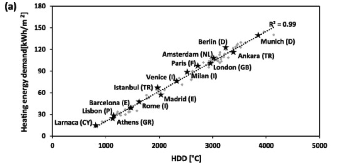
Relationship between heating demand and HDDaccording to De Rosa, Mattia, et al.
heating energy demand kWh/m2 = hdd * 0.042 - 21.8
3.2 Maintenance Costs
Climate change accelerates the wear and tear on physical assets. This metric focuses on the cumulative stress from chronic climate conditions — such as prolonged heat, persistent humidity, and total annual rainfall—which drives the need for increased routine maintenance. It quantifies the required increase in an annual maintenance budget to counteract this accelerated degradation using the formula below where the coefficients for each feature adjusts the actual impact for each unit of increase of the contributing features, giving an overall maintance increase value.
Maint_Increase = ∑(C_i ⋅ ΔFeature_i)
Which translates to: Maint_Increase = (C_heat ⋅ ΔDays>35C) + (C_humidity ⋅ ΔHigh_Humidity_Days) + (C_precip ⋅ ΔTotal_Annual_Precip) + (C_wind ⋅ ΔHigh_Wind_Days) + (C_freeze ⋅ ΔFreezeThaw)
Contributing Features:
| Feature (ΔFeature_i) | Description | Explanation | |
|---|---|---|---|
| ΔDays>35C | Change in the number of days with Tmax > 35°C | Increased heat places mechanical strain on systems and degrades materials like roofing and sealants. | Days |
| ΔHigh_Humidity_Days | Change in the number of days with avg. humidity > 70% | Persistent humidity accelerates corrosion on metal components and promotes costly mold growth. | Days |
| ΔTotal_Annual_Precip | Change in the total annual precipitation | Higher cumulative rainfall overloads drainage systems and accelerates the weathering of surfaces. | mm |
| ΔHigh_Wind_Days | Change in the number of days with avg. wind speed > 40 km/h | Frequent high winds cause mechanical fatigue on structural elements and force debris into systems. | Days |
| ΔFreezeThaw | Change in the number of annual freeze-thaw cycles | The expansion/contraction of water in cracks progressively destroys materials like concrete and asphalt. | Cycles |
Coefficients:
| Coefficient (C_i) | Description | Illustrative Value |
|---|---|---|
| C_heat | % budget increase per extra hot day | 0.002 (0.2%) |
| C_humidity_days | % budget increase per extra high-humidity day | 0.001 (0.1%) |
| C_precip | % budget increase per 100mm of extra annual rain | 0.005 (0.5%) |
| C_wind_days | % budget increase per extra high-wind day | 0.004 (0.4%) |
| C_freeze | % budget increase per extra freeze-thaw cycle | 0.003 (0.3%) |
Section 4 — Income
4.1 Operational Efficiency & 4.3 Workforce Productivity
| Feature | Description | Explanation | |
|---|---|---|---|
| ΔCDD | Change in annual Cooling Degree Days. | Increased cooling demand puts a direct energy load on cooling systems, reducing the net efficiency of some assets. | CDD |
| ΔHigh_Heat_Days | Change in the number of days per year with extreme heat conditions (e.g., Tmax > 35°C). | Extreme heat can reduce human labor productivity due to health risks and mandated work/rest cycles. | Days |
| ΔDry_Spell_Days | Change in the number of days per year that fall within a prolonged dry spell. | Water scarcity during dry spells can force a reduction in operational capacity for assets reliant on water. | Days |
4.2 Operational Downtime
Operational downtime is driven by the increased frequency of acute hazard events that force a temporary slowdown or complete shutdown of operations. This metric estimates the increase in the number of downtime days per year for a given location.
Formula: ΔDowntime_total = ∑(ΔHazard_Metric_i)
| Feature | Description | Rationale | |
|---|---|---|---|
| ΔHotdays40C | Change in annual days above 40 degrees celsius. | Outdoor labour hours during days above 40 degrees celsius are greatly reduced | |
| ΔHeavy_Precip_Days | Change in days per year where daily precipitation exceeds a historical baseline (e.g., 95th percentile). | Extreme rainfall can cause localized flooding, disrupting logistics, access, and site safety. | Days |
| ΔHigh_wind_days | Change in days with extreme wind events | Extreme wind events causes disruptions in outdoor work and logistics. | Index |
| ΔDry_Spell_Days | Change in the total number of days per year that fall within a prolonged dry spell (e.g., 14+ consecutive days with <1mm rain). | Extended dry spells can lead to water use restrictions or shortages, impacting operations. | Days |
Section 5 — CapEx
5.1 Retrofit Costs
Remediation measures are crucial to mitigate the increasing risks posed by climate change. For example, retrofitting homes to improve insulation and ventilation can significantly reduce cooling demand and enhance thermal comfort, thereby reducing energy consumption. Similarly, implementing flood defenses and fire-resistant materials can mitigate damage and lower insurance premiums.
The retrofit recommendations provide a general guideline on the retrofit expenditure required for assets to adapt to a changing climate as CapEx denominated as percentage of annual net income.
For each relevant climate risk category (i.e. Heat Stress, Flood, Fire), we find the difference of the Mean Damage Ratio between 2025 and 2050 and translate the difference to estimated CapEx based on an exponential scale of 0-10% as shown in the following table. In practice, the exact breakpoint is calculated dynamically for each hazard type using a min-max scaling function. For each risk category, the maximum additional CapEx is capped at 10% of income. If the asset is exposed to multiple risk categories, the additional CapEx for each risk is summed together, and can exceed 10%.
CapEx Tiers:
| Risk Damage % Difference | Required CapEx (%) | Example Retrofits |
|---|---|---|
| 10% | 1% | "Minor upgrades, improved seals, enhanced monitoring." |
| 30% - 50 % | 5% | "HVAC system upgrades, improved site drainage, backup power." |
| >50% | 10% | "Major structural reinforcement, flood walls, asset relocation." |
The following histogram shows the total additional CapEx for 1 million randomly selected assets around the world across all hazards. With the heavy-tail nature of the distribution, 50% of assets would experience an additional CapEx below 3.2% while highly exposed assets would require heavy investments of up to 14% in additional CapEx.
.png)
Histogram of the total additional capex based on future changes in risk profiles of 1 million random assets. The higher the CapEx, the higher the expected increase in the overall risk exposure of an asset.
All the metrics above can be easily incorporated into standard financial frameworks, including Discounted Cash Flow (DCF) models for climate-adjusted valuation.
The Average annual loss (AAL) can also be calculated by taking the annualized changes in NPV from the climate-adjusted valuation.
This article captures how these metrics come together to form a climate-adjusted valuation in a DCF model.